Hyperelastic Material Models

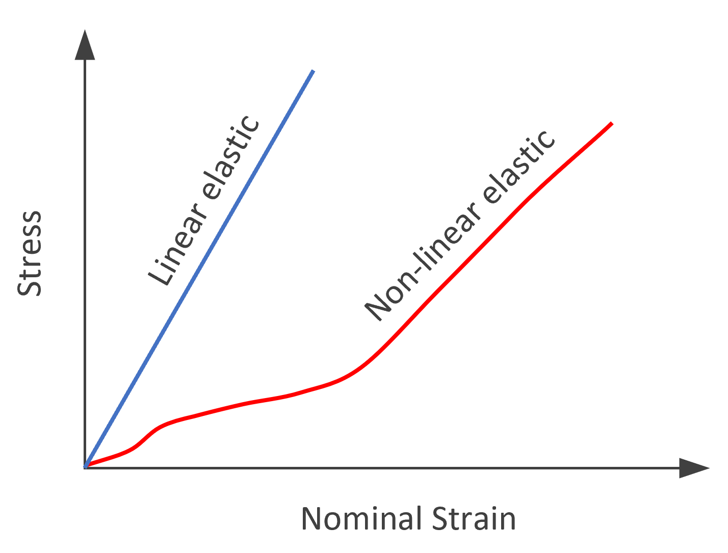
Lightly crosslinked polymers, also knowns as elastomers or rubbers, exhibit a highly non-linear stress-strain behavior, with extension values reaching up to 1000%. The typical elastomers are practically incompressible. However, unlike ordinary elastic materials, Hooke’s law is not applicable when describing the elastic response of an elastomer. The typical elastic stress-strain curves of linear elastic materials and of highly non-linear elastomers are schematically depicted in the figure on the right side.

The isotropic elastic properties of a hyperelastic materials can be derived from the strain energy density function, which defines the strain energy stored in the elastomer per initial unit volume. This function comprises the elastic deformation energy w_def and the energy stored due to volumetric changes w_vol:

where I₁, I₂ and I₃ are the Finger deformation tensor invariants and J is the determinant of the deformation tensor,

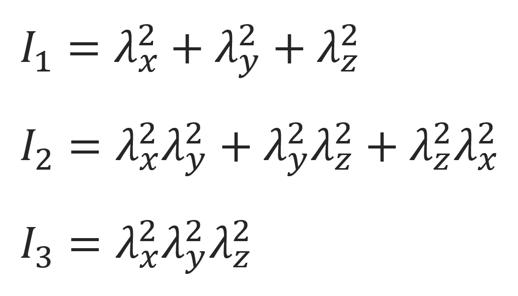
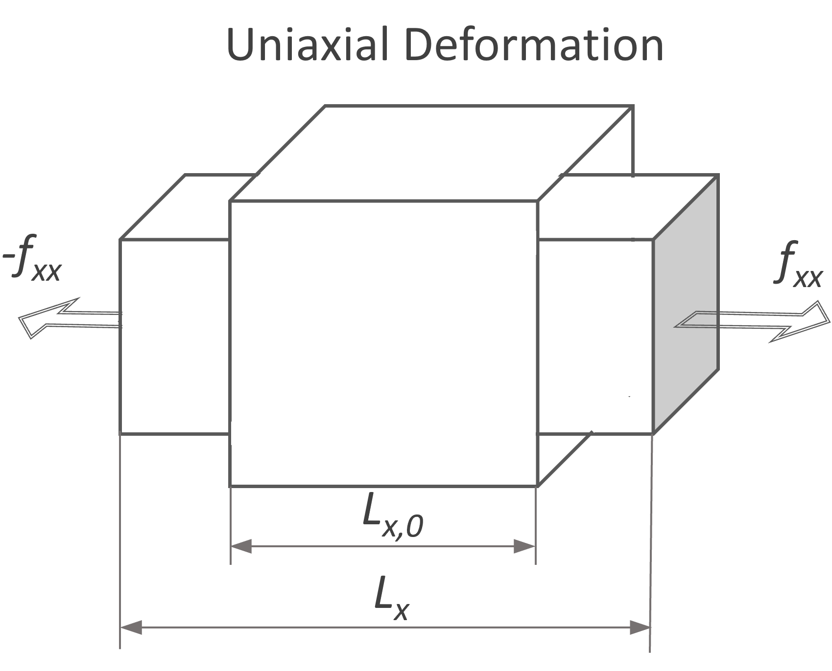
where λ_i = L_i / L_0,i are the principal stretch ratios, defined as the ratio of the length of a stretched line element to the length of the corresponding undeformed line element. In the case of an incompressible material, the third invariant is equal to one. Then the first and second invariant reduces to

Thus, invariants can be expressed as a function of only two stretch ratios

Calculating the mechanical behavior of rubbers in large deformation requires a number of mathematical theories of nonlinear, large elastic deformations. These theories combined with numerical methods such as Finite element analysis can be used by engineers to analyze and predict the response of elastomeric products operating under high strain. Almost all of these theories are based on the assumption that rubber is isotropic in elastic behavior and nearly incompressible. Below, four of the most popular hyperelastic material models, developed over five decades, are briefly discussed.

Generalized Rivlin Model

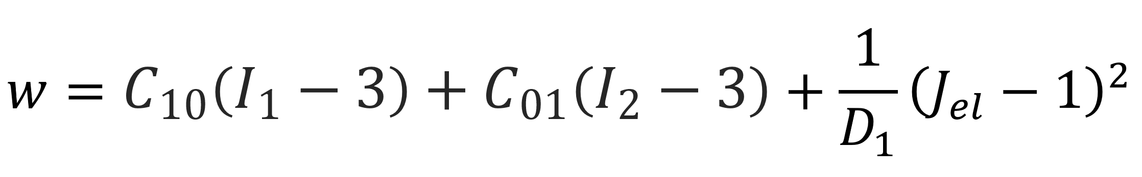
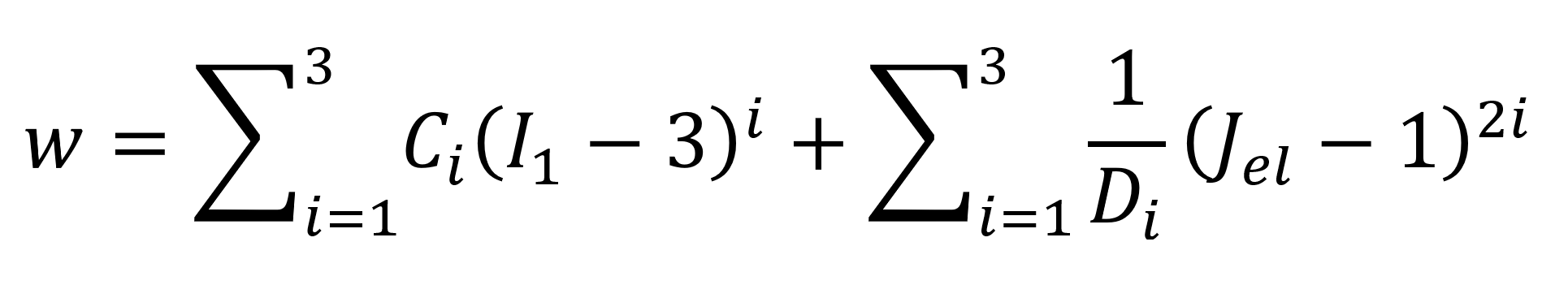
One of the oldest hyperelastic material model is the generalized Rivlin model, also known as the polynomial (hyperelastic) model.^1-3 It is expressed in terms of the two strain invariants I₁ and I₂ of the Finger stress tensor. With C_ij denoting material constants, its strain energy density reads

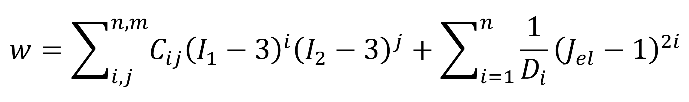
where C_ij and D_i are temperature-dependent parameters, and J_el is the elastic volume ratio. One of the most popular version of this model is based on a linear combination of the two invariants:

For an incompressible material, this equation simplifies to

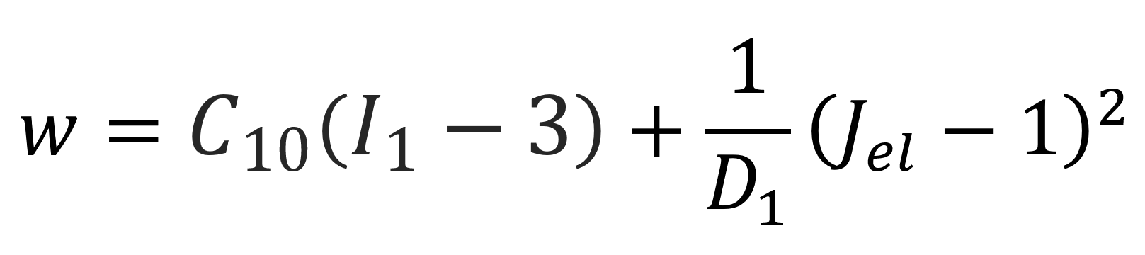
This version is known as the Mooney-Rivlin model since it was developed a few years earlier by Mooney (1940) and Rivlin (1948).^1,2 It can be derived from the Rivlin model by setting n = 1, C₁₀ = C₁, C₀₁ = C₂, and C₁₁ = 0. The polynomial model can be further simplified when setting C₀₁ = 0. The resulting model is the so-called Neo-Hookean Model, first proposed by Treloar in 1943:⁴

Ogden Model

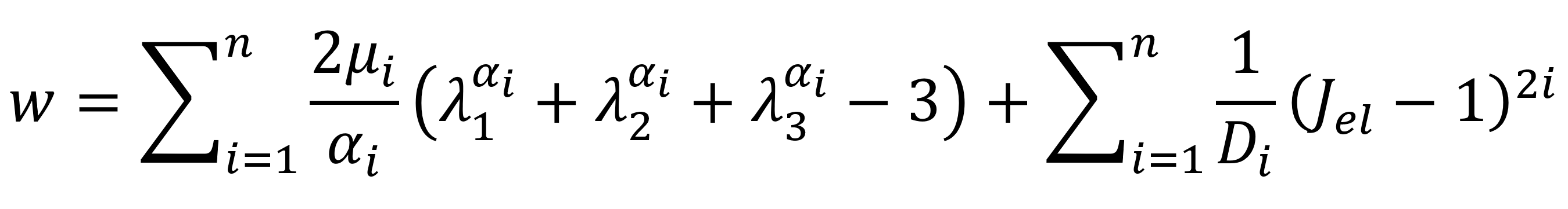
The Ogden model, first introduced in 1972, is one of the most widely used models.⁵ This model expresses the strain energy function w in terms of principal stretch ratios I₁, I₂ and I₃:

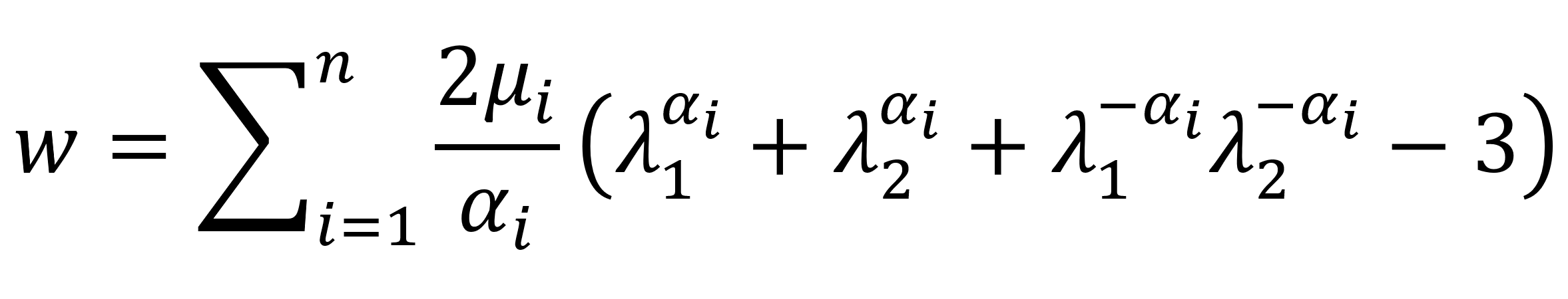
For incompressible materials (λ_xλ_yλ_z - 1 = 0) this equation can be rewrite as

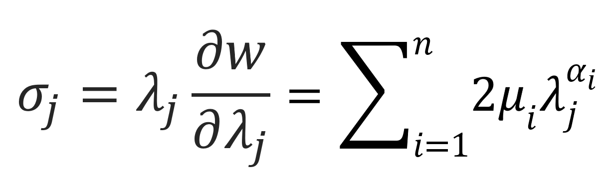
The three principal values of the Cauchy stresses can be obtained by performing the differentiation with respect to the extension:

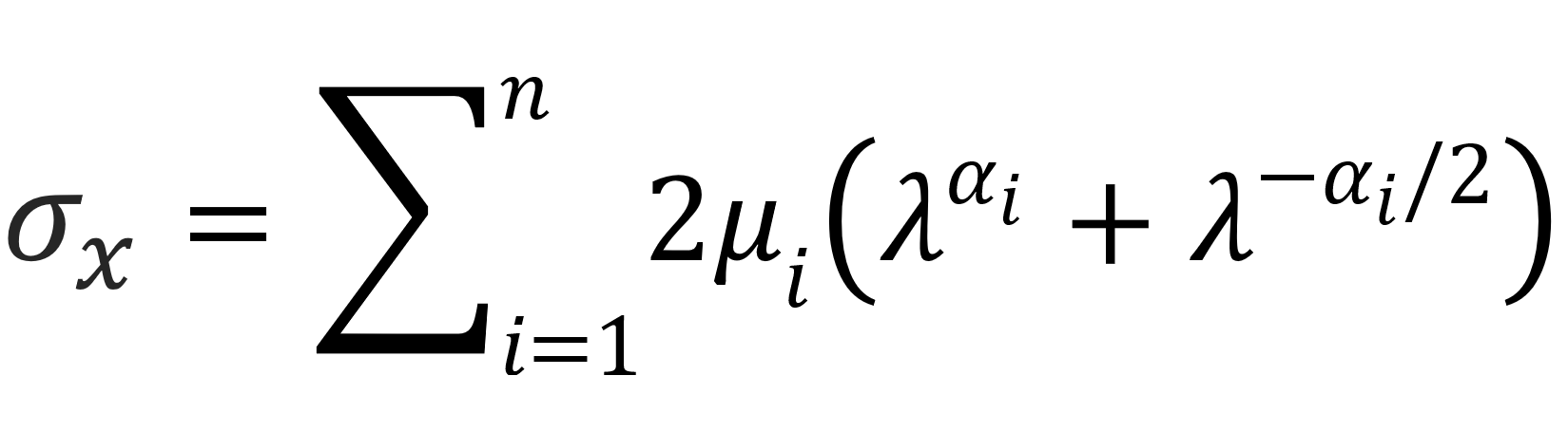
For an incompressible material under uniaxial tension (σ_y = σ_z = 0), the Ogden equation reads in terms of the extension ratios:

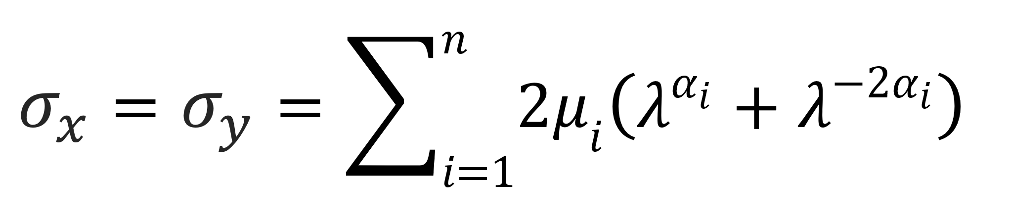
whereas for equi-biaxial tension (σ_x = σ_y, σ_z = 0) this reads

Yeoh Model

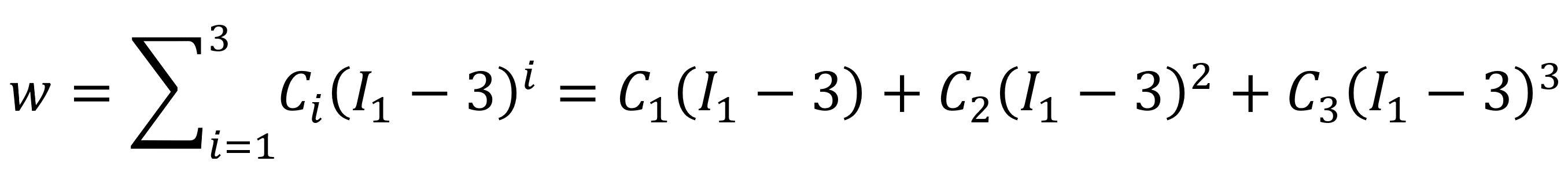
The Yeoh model,⁶ first introduced in 1990, is a special form of the reduced polynomial model with a three-term expansion (n = 3 and m = 0) and with only I₁ dependence

For incompressible materials, this equation reduces to

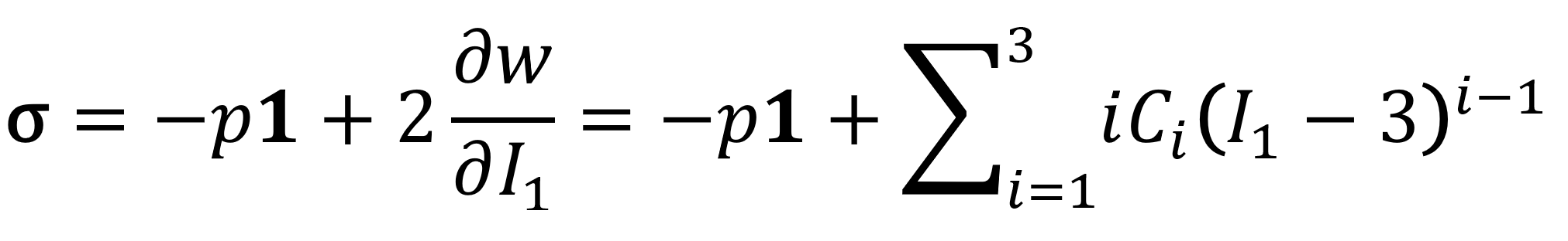
The Cauchy stress for incompressible hyperelastic materials is given by

This model can be applied to a wide range of deformation yielding reasonable results under large uniaxial stretching and simple shear deformation. However, when applied to more complex deformation containing different types of strains the Yeoh model may show inaccuracy.

For incompressible materials under uniaxial extension (σ_y = σ_z = 0):

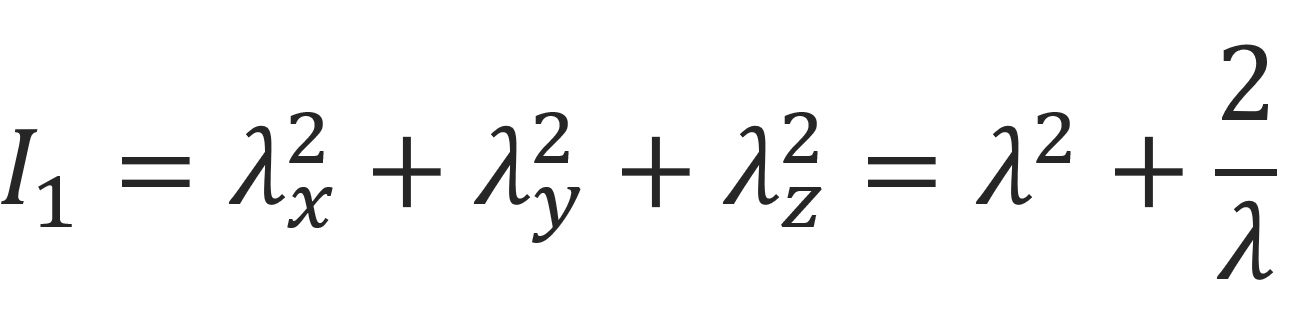
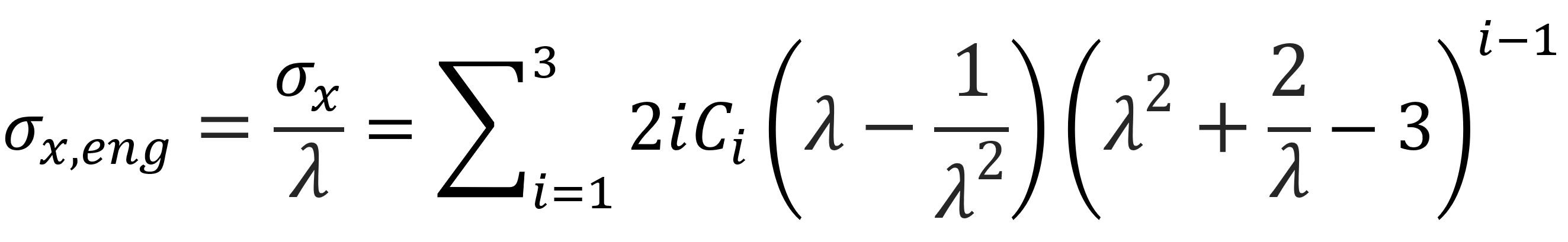
the Yeoh equation for stress reads

The engineering stress is

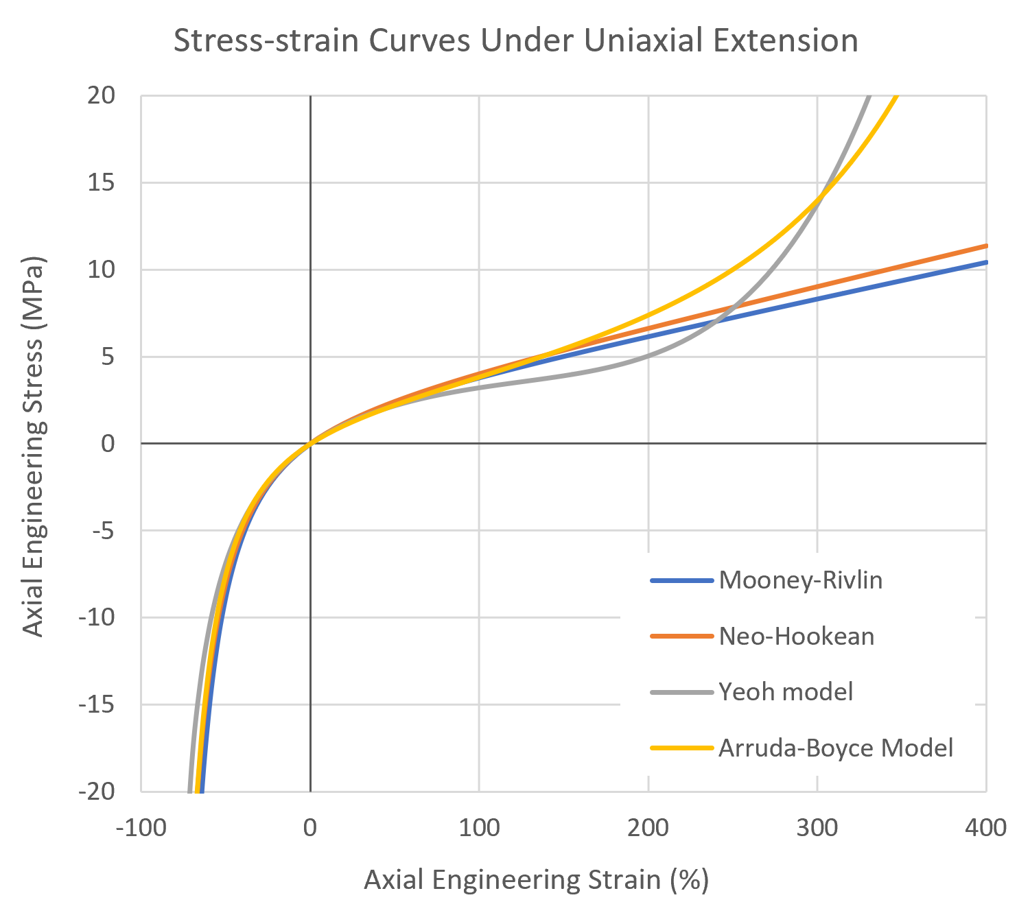
The figure below shows the stress-strain curves under uniaxial extension for the Yeoh model compared to the Neo-Hookean and Mooney-Rivlin models.¹² As can be seen, the latter two models have limitations for large strain, whereas more advanced models suchs as the Yeoh model and Arruda-Boyce model (see below) provide stress-strain curves with a much steeper slope at high deformations, which is a more realistic representation of the behavior of elastomers.

Arruda-Boyce Model

The Arruda-Boyce model was first introduced in 1993.⁷ It is based on an eight-chain network that considers eight orientations of chains in space with a non-Gaussian behavior of the individual sub-chains in the proposed network. Unlike most other hyperelastic materials models, it requires only two material parameters, an initial modulus and a limiting chain extensibility.

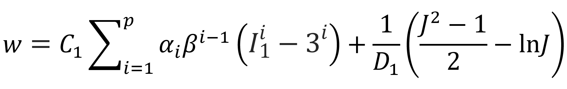
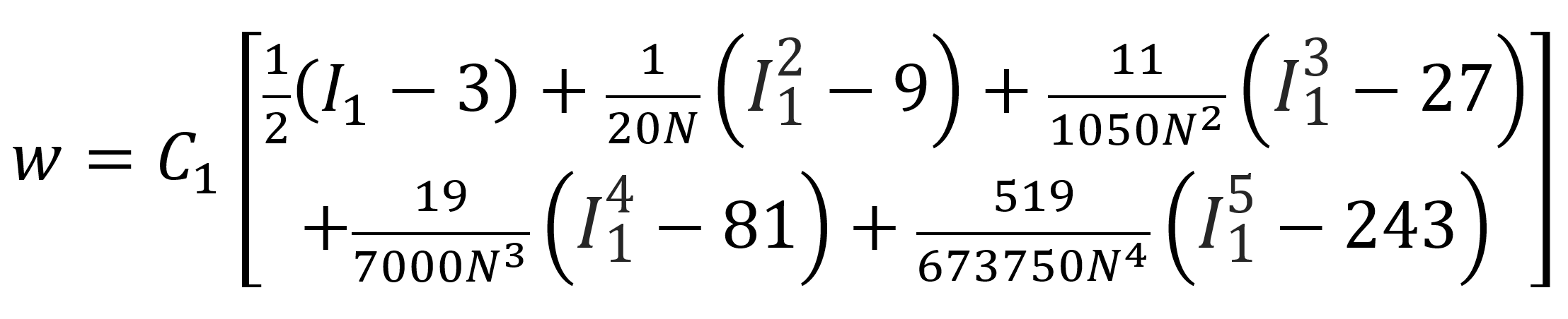
where C₁ = nkT is a material constant that can be expressed as the product of subchain density n, temperature T and Boltzman constant k, β = 1/N is the inverse of the number of statistical segments between crosslinks, J is the determinant of the strain gradient tensor and D₁ is another material constant related to the bulk modulus. The α_i are coefficients of the series expansion of the inverse Langevin function: α_1 = 1/2, α_2 = 1/20, α_3 = 11/1050, α_4 = 19/7000, α_5 = 519/673750. Assuming the rubber is incompressible, and using the first 5 terms of the inverse Langevin function, the strain energy density can be written as

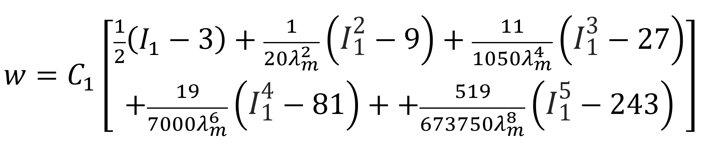
The initial chain length is assumed to be identical with that of a random walk of N steps of length l: r₀ = l N^1/2. The fully extended chain has the length l N. Then the limiting extensibility (or chain locking stretch), defined as the ratio of final length to initial length, is λ_m = N^1/2. Then the Arruda–Boyce model can be written in the form

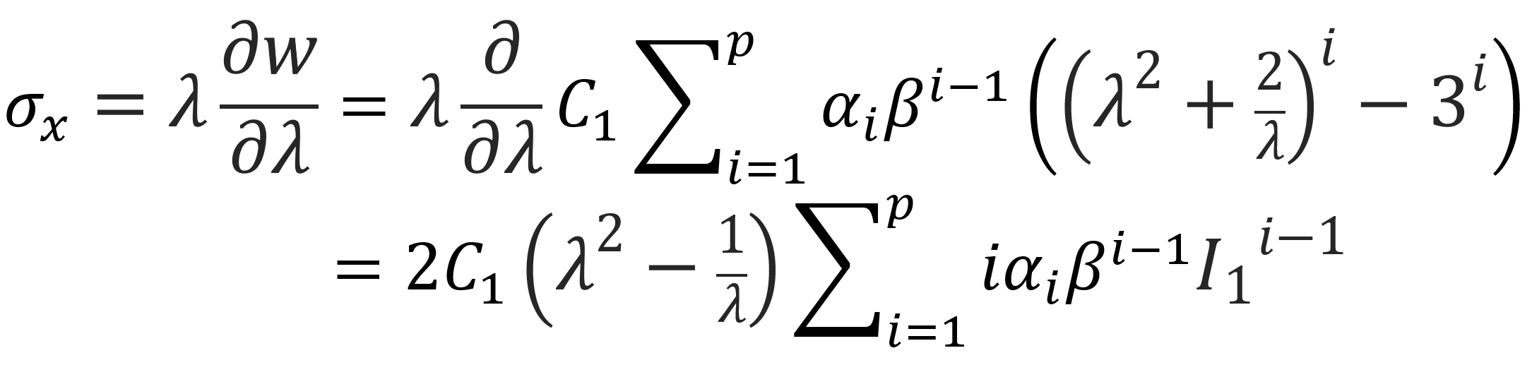
For incompressible materials under uniaxial extension, σ_y = σ_z = 0, the uniaxial stress σ_x can be obtained by differentiation with respect to the extension:

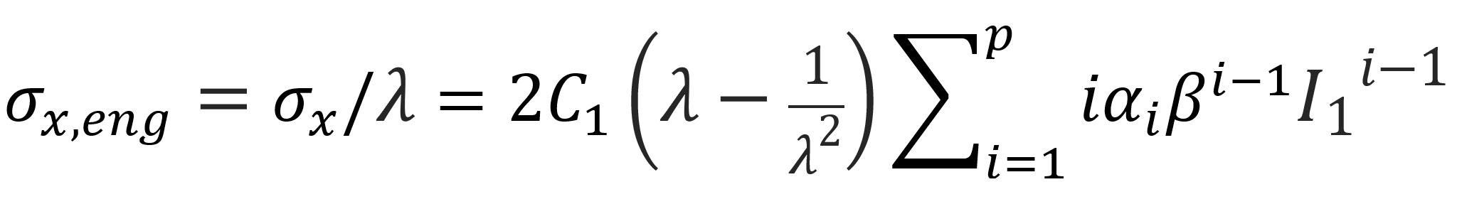
The engineering stress is

References & Further Reading

1. M. Mooney, J. Appl. Phys., Vol 11, 582-592 (1940)
2. R.S. Rivlin, Math. & Phys. Sci., Vol. 240 A, 491-508 (1948)
3. R.S Rivlin & D.W. Saunders. Philos. Trans. Royal Soc. A: Math. Phys. Eng. Sci., 243, 251 (1951)
4. L.R.G. Treloar, J. Chem. Soc., Faraday Trans., 39, 36‐41 (1943)
5. R.W. Ogden, Proc. R. Soc. Lond. A., 326, 565-584 (1972)
6. O.H. Yeoh, Rubber Chemistry and Technology, 63 (5), 792-805 (1990)
7. E.M. Arruda, M.C. Boyce, J. Mech. Phys. Solids, 41(2), 389‐412, (1993)
8. G. Strobl, The Physics of Polymers, 3rd Edition, Heidelberg 2007
9. M. Rubinstein and R. Colby, Polymer Physics, 1st Ed., Oxford University Press (2003)
10. L.R.G. Treloar, The Physics of Rubber Elasticity, Oxford 1949
11. They are called invariants because they do not change when the coordinate system is transformed (rotated).

12. The curves have been calculated with the parameters given in HandWiki-Physics